Tutorial 1: Landcover Classification using Landsat 8
Datasets
The dataset for this tutorial can be found in the raster4ml_data google drive repository.
Download the LC08_L1TP_137045_20210317_20210328_01_T1.tar.gz file and extract in the
data directory.
Import Modules
Import the necessary modules.
import os
import glob
from raster4ml.preprocessing import stack_bands
from raster4ml.plotting import Map
from raster4ml.features import VegetationIndices
from raster4ml.extraction import batch_extract_by_points
1. Stack the Bands
First we need to stack all the bands together and make a multispectral image file. The mutispectral image will contain several channels/bands representing reflectance information from different wavelengths. Since the test dataset is downloaded from a Landsat 8 satellite, there are total 11 bands. However, we will only use the first 7 bands as they can accurately define most of the surface objects in terms of reflectance.
To stack the seperate bands into one image, we need to define the paths of all the bands in chronological order (actually any order you want, but remember the orders for future reference).
# Filter all the files that ends with .TIF
image_dir = r'.\LC08_L1TP_137045_20210317_20210328_01_T1'

# Empty list to hold the first 7 bands' paths
bands_to_stack = []
# Loop through 7 times
for i in range(7):
    bands_to_stack.append(os.path.join(image_dir,
                                    f'LC08_L1TP_137045_20210317_20210328_01_T1_B{i+1}.TIF'))
bands_to_stack
['.\LC08_L1TP_137045_20210317_20210328_01_T1\LC08_L1TP_137045_20210317_20210328_01_T1_B1.TIF',
'.\LC08_L1TP_137045_20210317_20210328_01_T1\LC08_L1TP_137045_20210317_20210328_01_T1_B2.TIF',
'.\LC08_L1TP_137045_20210317_20210328_01_T1\LC08_L1TP_137045_20210317_20210328_01_T1_B3.TIF',
'.\LC08_L1TP_137045_20210317_20210328_01_T1\LC08_L1TP_137045_20210317_20210328_01_T1_B4.TIF',
'.\LC08_L1TP_137045_20210317_20210328_01_T1\LC08_L1TP_137045_20210317_20210328_01_T1_B5.TIF',
'.\LC08_L1TP_137045_20210317_20210328_01_T1\LC08_L1TP_137045_20210317_20210328_01_T1_B6.TIF',
'.\LC08_L1TP_137045_20210317_20210328_01_T1\LC08_L1TP_137045_20210317_20210328_01_T1_B7.TIF']
# Use the stack_bands function from raster4ml to do the stacking
stack_bands(image_paths=bands_to_stack,
            out_file=os.path.join(image_dir, 'Stack.tif'))
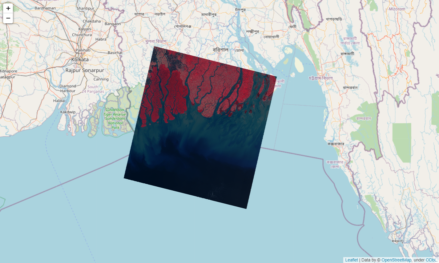
Let’s visualize the image using the plotting functionality of raster4ml.
# Define the map instance
m = Map()
# Add the raster to the map
m.add_raster(image_path=os.path.join(image_dir, 'Stack.tif'), bands=[4, 3, 2])
m
2. Calculate Vegetation Indices
In next step, we need to calculate the vegetation indices from the stacked image. We can do this using raster4ml.features.VegetationIndices object. You can provide a list of vegetation index we need to calculate in the object, but the tool can automatically calcualte all the possible vegetation index rasters.
To do this, we need to provide the path of the stacked image, the corresponding wavelength values and an output directory to save all the indices as rasters. Since this is a Landsat 8 OLI image, we know the band wavelengths. The wavelengths can be inserted as either the center_wavelengths as list or the range of wavelengths per band in a list of list. The wavelengths has to be specified in nanometers (nm). The Landsat 8 OLI wavelengths can be seen here.
Optionally we can provide the bit_depth as a parameter. Since we know Landsat 8 data is a 12-bit data, we can provide this information to normalize the image values from 0 to 1.
# Define the VegetationIndices object
VI = VegetationIndices(image_path=r'.\LC08_L1TP_137045_20210317_20210328_01_T1\Stack.tif',
                    wavelengths=[[430, 450], [450, 510], [530, 590], [640, 670], [850, 880], [1570, 1650], [2110, 2290]],
                    bit_depth=12)
# Run the process while providing the output directory
VI.calculate(out_dir=r'.\LC08_L1TP_137045_20210317_20210328_01_T1\VIs')
Calculating all features
100%|██████████| 354/354 [01:44<00:00,  3.40it/s]
311 features could not be calculated.
The reason 311 feature could not be calculated is that some of the vegetation indices require bands with more wavelengths than the wavelengths provided in the test image. Probably using a hyperspectral image that has bands from VNIR to SWIR, could reveal all the vegetation indices.
3. Extract Values based on Sample Points
Locate the sample point shapefile in the extracted data folder. The name of the shapefile
is points.shp. We need to extract the vegetation index values underneath each point in
the shapefile and store those index values for Machine Learning training. The shapefile
also contains label information. For simplicity, it only has two distinct classes, i.e.,
Vegetation and Water.
For extraction by points, we can use the raster4ml.extraction.batch_extract_by_points
function. This will enable extraction of multiple raster data at once. The function takes
image_paths as a list, shape_path as a string, and a unique_id in the
shapefile which uniquely represent each point. The function returns a pandas dataframe.
# Find the paths of all the vegetation indices
vi_paths = glob.glob(r'.\LC08_L1TP_137045_20210317_20210328_01_T1\VIs\*.tif')
# Batch extract values by points
values = batch_extract_by_points(image_paths=vi_paths,
                                 shape_path=r'.\LC08_L1TP_137045_20210317_20210328_01_T1\shapes\points.shp',
                                 unique_id='UID')
100%|███████████████████████████████████████████████████████████████████████████████████████████████████████| 48/48 [00:29<00:00,  1.62it/s]
6 columns were removed from the dataframe as they had duplicated values.
The VIs can have duplicate values because sometimes the equation will not end up with mathematical errors, but result in flat constant raster. That raster is not useful for any machine learning operation. Therefore the batch extract function automatically finds out those VIs and remove from the analysis.
4. Machine Learning Training
Now that we have our data ready, let’s build our machine learning model pipelines. We will
explore two machine learning models, i.e., Support Vector Machine (SVM) and Random Forest
(RF) classification here. Our target variable can be found in the point shapefile as the
Label column. The independent variables will be the vegetation index values calculated
in the last step.
We will utilize functionalities from scikit-learn to train the models. scikit-learn
has an automatic pipeline feature that performs several tasks at once. Machine
learning models also require hyperparameter tuning to fine tune the model.
scikit-learn has a fetaure for automatically doing that as well using GridSearchCV.
We will employ all these steps at once using the pipeline.
Therfore install the scikit-learn using either pip or conda in the same
environment and import the following modules.
from sklearn.model_selection import train_test_split
from sklearn.preprocessing import MinMaxScaler
from sklearn.pipeline import Pipeline
from sklearn.model_selection import GridSearchCV
from sklearn.svm import SVC
from sklearn.ensemble import RandomForestClassifier
from sklearn.metrics import accuracy_score

import geopandas as gpd
import numpy as np
# Read the shapefile to get the points shapefile
# Note that the rows of this shapefile and the extracted values match
shape = gpd.read_file(r".\LC08_L1TP_137045_20210317_20210328_01_T1\shapes\points.shp")
First, we need to split the dataset into training and testing set.
X_train, X_test, y_train, y_test = train_test_split(values, shape['Label'].values,
                                                    test_size=0.3,
                                                    random_state=42)
print('X_train shape:', X_train.shape)
print('X_test shape:', X_test.shape)
print('y_train shape:', y_train.shape)
print('y_test shape:', y_test.shape)
X_train shape: (70, 42)
X_test shape: (30, 42)
y_train shape: (70,)
y_test shape: (30,)
Then, we just need to define the Pipeline, GridSearchCV and the model to do the
training.
## Support Vector Machine

# Define pipeline
pipe_svc = Pipeline(steps=[('scaler', MinMaxScaler()), # Scaling the data from 0 to 1
                        ('model', SVC())])

# Define pipeline parameters
# Note that we are only testing 2 hyperparameters, you can do even more or expand the search
param_svc = {'model__gamma': [2**i for i in np.arange(-10, 7, 1, dtype='float')],
            'model__C': [2**i for i in np.arange(-10, 7, 1, dtype='float')]}

# Define grid
grid_svc = GridSearchCV(estimator=pipe_svc,
                        param_grid=param_svc,
                        cv=5, # 5-fold cross validation
                        n_jobs=4) # Paralelly using 4 CPU cores
grid_svc.fit(X_train, y_train)
## Random Forest Classifier

# Define pipeline
pipe_rfc = Pipeline(steps=[('scaler', MinMaxScaler()), # Scaling the data from 0 to 1
                        ('model', RandomForestClassifier())])

# Define pipeline parameters
# Note that we are only testing 2 hyperparameters, you can do even more or expand the search
param_rfc = {'model__n_estimators': [2**i for i in range(5)],
            'model__max_features': ['sqrt', 'log2']}

# Define grid
grid_rfc = GridSearchCV(estimator=pipe_rfc,
                        param_grid=param_rfc,
                        cv=5, # 5-fold cross validation
                        n_jobs=4) # Paralelly using 4 CPU cores
grid_rfc.fit(X_train, y_train)
Now that we have trained two models, lets check the accuracy score from both models. We
can directly use the grid objects. If we directly predict from the grid object,
then it picks out the model with the best hyperparameters and use that for prediction.
You can also go into the grid object and examine which model to pick and so on. Please
refer this link to learn more.
# Predict the test set
y_pred_svc = grid_svc.predict(X_test)
y_pred_rfc = grid_rfc.predict(X_test)
print(f"Accuracy from SVC: {accuracy_score(y_test, y_pred_svc):.2f}")
print(f"Accuracy from RFC: {accuracy_score(y_test, y_pred_rfc):.2f}")
Accuracy from SVC: 0.97
Accuracy from RFC: 1.00